Economics
3343: Course Project
Dr. Philip Rothman
Office: Brewster A-424
Phone: 328-6151
Email: rothmanp@ecu.edu
Due date/time: Thursday, May 9, 8am. A hard copy of the paper needs to be submitted upon your arrival
for the Final Exam; submission by e-mail will NOT be accepted; if you wish,
you may submit the paper before the due date/time.
I. Topical Focus
Your project will be based upon analysis of a
set of estimated regression models motivated by what is known as the Capital
Asset Pricing Model (CAPM). I have provided a Brief
Introduction to the CAPM and Factor Models, with an emphasis on some key
econometric issues; you are STRONGLY ENCOURAGED to
read through and ‘digest’ that material ASAP. The remainder of this document
assumes you indeed are sufficiently familiar/comfortable
with that material.
II. Data
Each student will use the following data to
estimate the CAPM and factor models:
1.
The excess return on the ‘market portfolio’ (![]() ) from the Fama
and French Data Library.
) from the Fama
and French Data Library.
2.
The ‘change in risk premium’ (![]() ) measure given by the difference between the yields on Baa and Aaa rated bonds.
) measure given by the difference between the yields on Baa and Aaa rated bonds.
3.
The ‘small minus big’ (![]() ) measure from the Fama
and French Data Library.
) measure from the Fama
and French Data Library.
4.
The ‘high minus low (![]() ) measure from the Fama
and French Data Library.
) measure from the Fama
and French Data Library.
Note: various combinations of the above data
will be used as the INDEPENDENT or EXPLANATORY variables in your estimated regression models. You can download
these data in an EViews workfile
by CLICKING HERE. The EViews variable names for these data are: ‘er_mkt’ for the excess return on the market portfolio; ‘crp’ for the change in risk premium; ‘smb’
for the ‘small minus big’ size premium measure; and ‘hml’
for the ‘high minus low’ size premium measure. Note that these are monthly data
and the sample period starts in July of 2001 and ends in December of 2012.
Each student has been assigned a different stock (a
‘security’ in the language of CAPM and factor models), such that each of you
will be using different data for the DEPENDENT variable in your regression
models. Each of these securities is a component of the S&P500 stock index.
To see which stock you have been assigned, CLICK HERE. The link associated with your
name will take you to a Yahoo Finance web
site at which you can download the historical data you will need. Once you are
at this site:
1. For the ‘Start Date,’ you should
enter ‘June 1, 2001’
2. For the ‘End Date,’ you should
enter ‘December 31, 2012’
3. You should indicate that you want
‘Monthly’ data
4. After you have specified these
parameters, scroll down and click on the ‘Download to Spreadsheet’ link. This
will allow you to download your download into a ‘Comma-Separated-Value’ (with
the extension ‘csv) file which can be opened with
Excel. CLICK HERE to see such a file with data on the ExxonMobil Corporation’s stock
price. For a student assigned ExxonMobil’s stock for this project, the data
series needed for the assignment would be in the last column under the heading
‘Adj Close’ (for ‘adjusted closing price,’ where the
price at the end of trading is adjusted for dividends and stock splits.
Below is an
explanation of how you need to transform such data for use in the project:
1. Delete all the columns from the initial
file except the first one (with the dates) and the last one (with the ‘Adj Close’) data. For an example, CLICK HERE; note that the initial CSV file
has been saved into an Excel file. Note: when you create an Excel file, make sure to save
it as an ‘Excel 97-2003 Workbook’ (i.e., with an ‘xls’
extension, not an ‘xlxs’ extension).
2. Next, arrange the data in
chronological order, i.e., oldest to newest. To do so, highlight all data cells
in the file, then left click, then click on Column
> Sort by ‘Date’, Sort On >
Values, ‘Sort,’ and then Order > ‘Oldest
to Newest. To see what you get after doing this, CLICK HERE.
3. Next, compute the month-to-month
growth rate in the ‘Adj Close’ measure. An easy way
to do this would be to copy the formula in cell ‘C3’ from THIS FILE, paste it in your file, and then
use it fill out the cells ‘C3-C140’ in your file. The variable name ‘r’ in cell
‘C1’ stands for the rate of return on the stock/security you’ve been assigned.
4. Next, copy the data for the
variable ‘rf’ (the ‘risk-free rate’ measure from the Fama
and French Data Library) from
column ‘D’ in THIS
FILE and past the
copied data into column ‘D’ in your file (starting in cell D3).
5. Next, for each row, subtract the
entry from the cell in column ‘D’ from the entry for the cell in column ‘C,’ as
done in THIS FILE. Note that this computes the
‘risk premium’ for the stock; the name in cell ‘E1,’ ‘er_r,’
is meant to indicate the excess return on the stock/security you’ve been
assigned computed using the rate of return on the stock/security.
6. Next, highlight cells ‘E1’ to
‘E140,’ right-click and then click on ‘Copy,’ then place the cursor on cell
‘E1,’ right-click and then click on ‘Paste Special’ and then under ‘Paste’
click on ‘Values’ and then ‘OK.’ Then delete columns ‘B ‘
through ‘D’; and also delete Row 2. Then replace the entries in Column
‘A’ with the Column ‘A’ from THIS FILE.
7. Finally, enter the data you have
computed for the stock’s excess return into EViews by
following these steps: (a) open THIS EViews WORKFILE
in EViews; (b) left-click File
> Import > Read Text-Lotus-Excel, then go to the folder where the
Excel file with your ‘er_r’ data is located and click
on the file to indicate to EViews that this is the
file you want to import (note: make sure the Excel file is NOT open in Excel);
(c) in the EViews window that opens, the ‘upper-left
data cell’ should be ‘B2’ and, in the ‘Names for series or Number if names in
file’ box, enter ‘1’ and then hit the ‘OK’ button. Now the series ‘er_r’ will also be in the file.
Now you have
data with which you can estimate equations (3), (6), (7), and (8), i.e.,
equations for the CAPM and the factors models discussed HERE.
III. Econometric Tasks
1. Estimate the CAPM equation (3) by
OLS. [You can do this in EViews as follows: (a) put the cursor on the command line
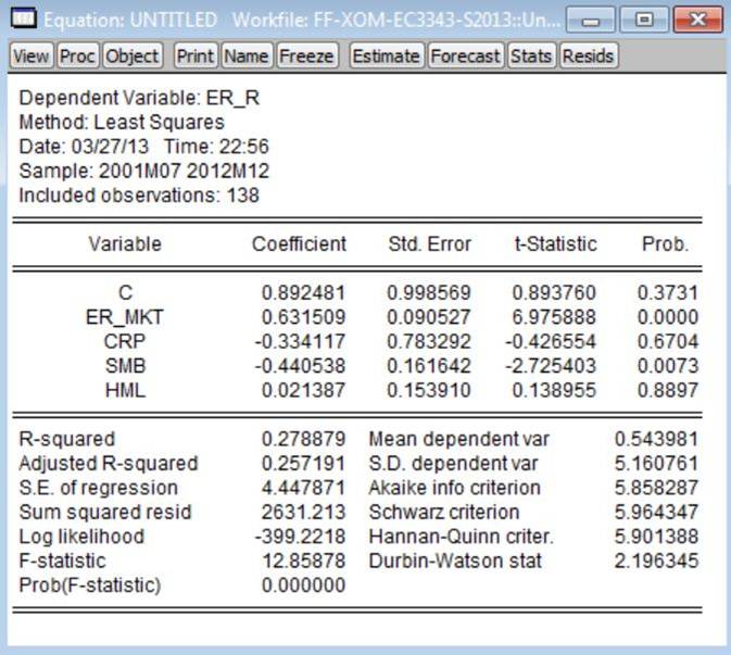
(top-left corner of screen); (b) type: ls er_r c er_mkt; (c) hit the ‘Enter’ key.] Refer to this as ‘Model 1.’ Using the Exon Mobil excess returns data
as the dependent variable, the estimated version of Model 1 is:
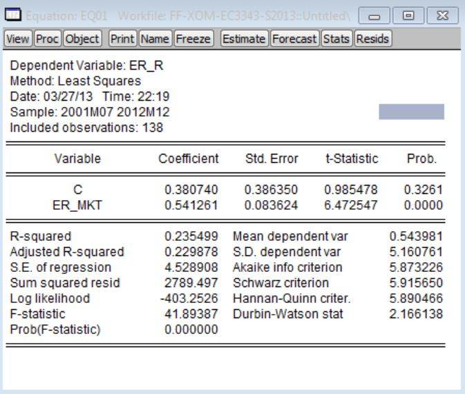
Note:
After this model has been, you should left-click on Name > OK; make sure to do this for all of the estimated models
for this project. The default name for the first estimated model stored in a workfile is ‘eq01’. You should also make sure to save your workfile.
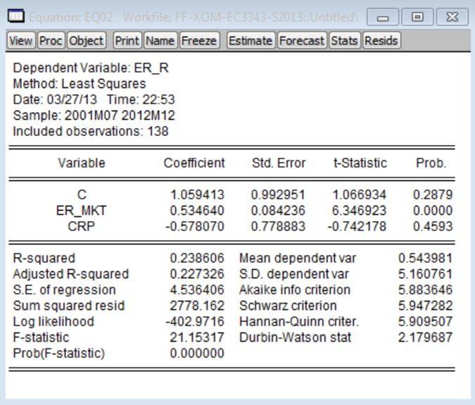
2. Estimate equation (6) by
OLS. [You can do this in EViews as
follows: (a) put the cursor on the command line (top-left corner of screen);
(b) type: ls er_r c er_mkt crp; (c) hit the ‘Enter’ key.] Refer to this as ‘Model 2.’
Using the Exon Mobil excess returns data as the dependent variable, the
estimated version of Model 2 is:
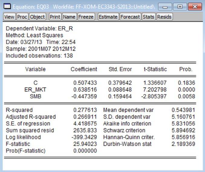
3. Estimate the model given by
adding the ‘small minus big’ variable to equation (3). [You can do this in EViews
as follows: (a) put the cursor on the command line (top-left corner of screen);
(b) type: ls er_r c er_mkt smb; (c) hit the ‘Enter’ key.] Refer to this as ‘Model 3.’ Using the Exon Mobil excess returns data
as the dependent variable, the estimated version of Model 3 is:
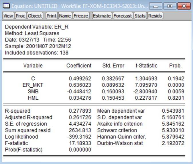
4. Estimate the model given by
adding the ‘high minus low’ variable to equation (3). [You can do this in EViews
as follows: (a) put the cursor on the command line (top-left corner of screen);
(b) type: ls er_r c er_mkt hml; (c) hit the ‘Enter’ key.] Refer to this as ‘Model 4.’ Using the Exon Mobil excess returns data
as the dependent variable, the estimated version of Model 4 is:

5. Estimate the three-factor model
given by equation (7). [You
can do this in EViews as follows: (a) put the cursor
on the command line (top-left corner of screen); (b) type: ls er_r c
er_mkt smb hml; (c) hit the ‘Enter’ key.] Refer to this as ‘Model 5.’
Using the Exon Mobil excess returns data as the dependent variable, the
estimated version of Model 5 is:
6. Estimate the four-factor combined
model given by equation (8). [You
can do this in EViews as follows: (a) put the cursor
on the command line (top-left corner of screen); (b) type: ls er_r c
er_mkt crp smb hml; (c) hit the ‘Enter’ key.] Refer to this as ‘Model 6.’ Using the Exon Mobil excess returns data
as the dependent variable, the estimated version of Model 6 is:
7. For each estimated model, test
the null hypothesis of no positive serial correlation against the alternative
hypothesis of positive serial correlation at the 5% significance level with the
Durbin-Watson test. Let’s see how this is done for the estimated version of
Model 1 above, for which the Durbin-Watson statistic = 2.166. Since a 1-sided
test is being run at the 5% significance level, the critical values ![]() and
and ![]() need to be obtained from Table 4 of the
‘Statistical Tables’ appendix. For all of the estimated regression models in
this project, the sample size is 138 (see ‘Included observations’ in the EVIews output). But note that the highest value of ‘N’
listed in Table 4 is 100. For the purposes of this project, we’ll use the
critical values associated for the N=100 case. For Model 1, K=1, so we use the
following critical values:
need to be obtained from Table 4 of the
‘Statistical Tables’ appendix. For all of the estimated regression models in
this project, the sample size is 138 (see ‘Included observations’ in the EVIews output). But note that the highest value of ‘N’
listed in Table 4 is 100. For the purposes of this project, we’ll use the
critical values associated for the N=100 case. For Model 1, K=1, so we use the
following critical values: ![]() and
and ![]() . Since DW = 2.166 > and
. Since DW = 2.166 > and ![]() , the decision rule for this test
implies that the null hypothesis is not rejected at the 5% significance level.
, the decision rule for this test
implies that the null hypothesis is not rejected at the 5% significance level.
8. For the estimated Models 1
through 6, run the hypothesis tests specified in items I-VI found on p. 3 of THIS FILE. Note that p-values for all but one of these null hypotheses (i.e., the
one for hypothesis test III) are provided in the standard regression output
produced by EViews. So, to “run” these tests after the
models have been estimated, there’s nothing to do other than to properly
interpret the associated p-values. To
run hypothesis test III, assume that, as in the EViews
examples highlighted above,
the opening ‘ls er_r’ is always followed by ‘c er_mkt’ (and other dependent variable names in Models 2-6), i.e., after
telling EViews to run an OLS regression with ‘er_r’ as the dependent variable, a constant is specified and then ‘er_mkt’ is listed as the first independent variable. Then, once the model has
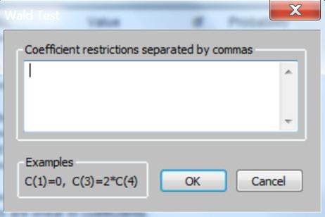
been estimated, do the following: click on View
> Coefficient Tests > Wald – Coefficient Restrictions. Then this
window will open up:
In the window enter: ‘c(2)=1’, as in:
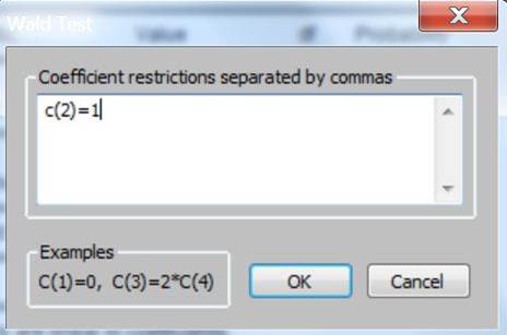
The ‘c’ refers to the an EViews variable that stores
the estimated coefficients; the ‘2’ tells EViews that the test is to be
run on second coefficient stored in ‘c’; the first coefficient stored in ‘c’ is the estimated constant term. Doing
this test for the estimated version of Model 1 using the excess returns data on
ExxonMobil’s stock leads to this (without the three red rectangles):
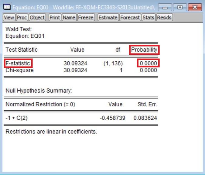
In the column labeled ‘Probability’ are p-values (for two approaches for
computing the p-value for this test).
You should use the p-value associated
with the ‘F-statistic’. Note: what EViews calls a
‘Wald Test’ is the ‘general F-test’
discussed in the appendix to Chp. 5 of the text.
Note: Suppose you’ve estimated Models 1 through 6 and stored the
estimated equations as ‘eq01’, ‘eq02’, …, ‘eq06’. You can
run hypothesis test III by first left-clicking on the particular equation name,
then clicking on View > Coefficient
Tests > Wald – Coefficient Restrictions, and running through the steps
given above.
9. For Models 5 and 6, test ![]() . Assuming these models have been
estimated with these exact commands, ‘ls er_r c er_mkt smb
hml’ and ‘ls er_r c er_mkt crp
smb hml’,
respectively, for Model 5 and Model 6. Assume Model 5 is stored in your workfile as
‘eq05’. Left-click on ‘eq05’ and then left-click on View > Coefficient Tests > Wald – Coefficient Restrictions to
get this window again:
. Assuming these models have been
estimated with these exact commands, ‘ls er_r c er_mkt smb
hml’ and ‘ls er_r c er_mkt crp
smb hml’,
respectively, for Model 5 and Model 6. Assume Model 5 is stored in your workfile as
‘eq05’. Left-click on ‘eq05’ and then left-click on View > Coefficient Tests > Wald – Coefficient Restrictions to
get this window again:
Then enter ‘c(3)=c(4)=0’ to test ![]() for Model 5. Next, Assume Model 6 is stored in your workfile as ‘eq06’. Left-click on ‘eq06’ and then
left-click on View > Coefficient Tests
> Wald – Coefficient Restrictions to get this window again:
for Model 5. Next, Assume Model 6 is stored in your workfile as ‘eq06’. Left-click on ‘eq06’ and then
left-click on View > Coefficient Tests
> Wald – Coefficient Restrictions to get this window again:
Then enter ‘c(4)=c(5)=0‘ to test ![]() for Model 6.
for Model 6.
10. For Model 6, test
![]() . Assume this model has been estimated with the command ‘ls er_r c
er_mkt crp smb hml’ and that the estimated model is stored as
‘eq06’. Left-click on
‘eq06’ and then left-click on View >
Coefficient Tests > Wald – Coefficient Restrictions to get this window
again:
. Assume this model has been estimated with the command ‘ls er_r c
er_mkt crp smb hml’ and that the estimated model is stored as
‘eq06’. Left-click on
‘eq06’ and then left-click on View >
Coefficient Tests > Wald – Coefficient Restrictions to get this window
again:

Then enter ‘c(3)=c(4)=c(5)=0‘ and click on ‘OK’ to test ![]() for Model 6.
for Model 6.
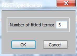
11. Run the RESET test for each model. Suppose you’ve estimated Models 1
through 6 and stored the estimated equations as ‘eq01’, ‘eq02’,
…, ‘eq06’. You can run the RESET test
by first left-clicking on the particular equation name, then clicking on View > Stability Tests > Ramsey RESET
Test, entering ‘3’ for the number of ‘fitted terms’ when this window pops
up:
and then clicking ‘OK’. Doing this for Model 1 estimated with the Exon
Mobil excess returns data as the dependent variable generates these results:
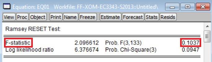
For your project, you should report the p-value associated with the ‘F-Statistic’ version of the RESET test.
12. Report your results for all of
the above in a table. If you click HERE,
you can download a WORD file with a table reporting such results for Models 1
through 6 estimated using the ExxonMobil excess returns stock data as the
dependent variable. You can use this WORD file as a template.
13. Run Bias Checks for each of the explanatory variables in Models 2
through 6, examine the effect (on the slope coefficients for other independent
variables) of dropping the variable from the model; discussion of this analysis
should be included in your paper. These are the particular bias checks you should examine:
a. Dropping ‘er_mkt’
from Model 2.
b. Dropping ‘er_mkt’
from Model 3.
c. Dropping ‘er_mkt’
from Model 4.
d. Dropping ‘er_mkt’
from Model 5.
e. Dropping ‘er_mkt’
from Model 6.
f.
Dropping ‘crp’ from Model 2.
g. Dropping ‘crp’
from Model 6.
h. Dropping ‘smb’
from Model 3.
i.
Dropping ‘smb’ from Model 5.
j.
Dropping ‘smb’ from Model 6.
k. Dropping ‘hml’
from Model 4.
l.
Dropping ‘hml’ from Model 5.
m. Dropping ‘hml’
from Model 6.
To
help analyze these results, it will be useful to have information on the
estimated correlations between the different independent variables. To produce
this information, first create an EViews ‘group’ with
the variables ‘er_mkt’, ‘crp’,
‘smb’, and ‘hml’. Then
click View > Covariance Analysis.
When this window opens up:
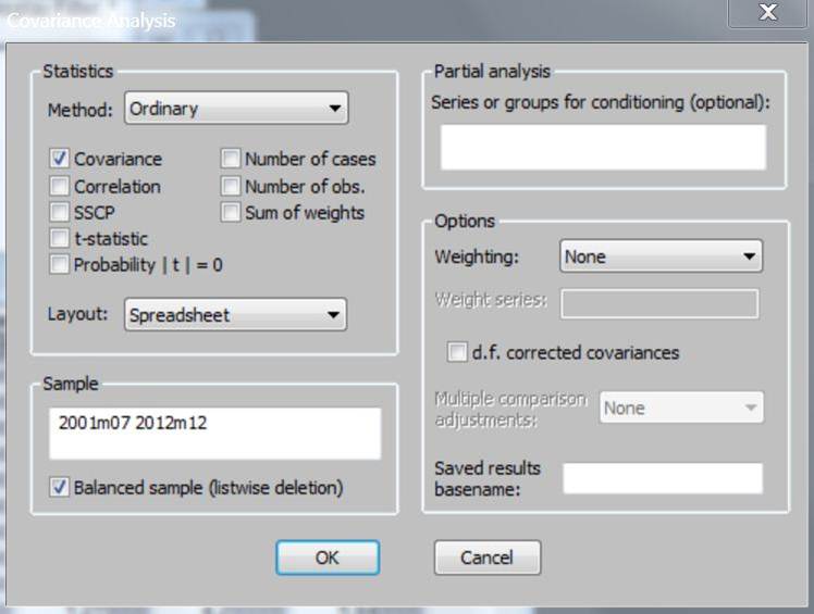
uncheck ‘Covariance’, check ‘Correlation’, on the ‘Layout’
table click ‘Single table’, and then click on ‘OK’. This window will then pop
up:
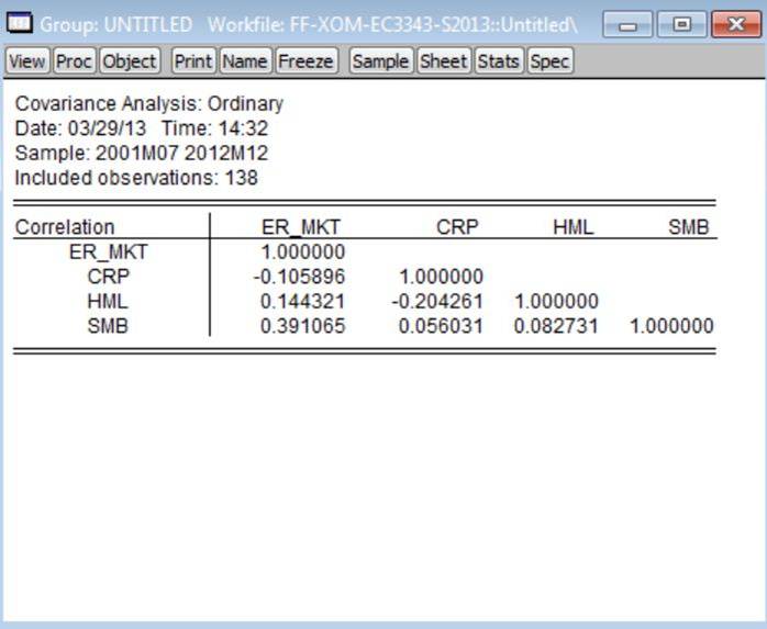
From
this table, we see the following sample correlation coefficients: (a) corr(er_mkt, crp) = -0.11; (b) corr(er_mkt, hml)
=0.14; (c) corr(er_mkt, smb) = 0.39; (d) corr(crp, hml) = -0.20; (e) corr(crp, smb)
=0.06; and (f) corr(hml, smb) = 0.08.
14. Based upon the results you obtain
and the underlying economic theory, determine which of the models you have
estimated is the ‘best’ model. In making this judgment, you should consider at
least the following criteria (which you might want to consider, along with
steps above, as part of the ‘rubric’ for this project):
a)
t-Test:
Is the variable’s estimated coefficient significant (at conventional
significance levels) in the expected direction?
b)
F-Test:
Is the variable’s estimated coefficient jointly (i.e., along with the
other estimated slope coefficients in the equation) significantly different
from zero (at conventional significance levels)?
c)
R-Bar-Squared: Does the overall fit of the
equation (adjusted for degrees of freedom) improve when the variable is added
to the model?
d)
Bias Check:
Do other variables’ coefficients change significantly when the variable
is added/deleted from the equation?
e) RESET Test: Does the RESET Test fail
to reject the null of no specification error when the variable is added to the
equation?
IV. Paper
Write a
paper describing what you have done and analyzing your results. Some specifics:
·
Your paper
should have at least three sections: ‘Section 1: Introduction’; ‘Section 2:
Analysis’; and ‘Section 3: Conclusions’; make sure your paper has a title page
and that, if your paper is not presented in a special report-type folder, all the pages are
stapled together (if they
are not stapled, your paper will not be accepted).
·
As part of
your analysis, it would be interesting to discuss the values of ![]() relative to 1. For example,
for all of the estimated Models 1 through 6 using the ExxonMobil excess returns
data at the dependent variable, of
relative to 1. For example,
for all of the estimated Models 1 through 6 using the ExxonMobil excess returns
data at the dependent variable, of ![]() < 1, implying that the
returns for this stock are less volatile than returns on the overall market.
Does this make sense? It’s a ‘BLUE CHIP’
stock that’s one of the components of the DOW
JONES INDUSTRIAL AVERAGE that has a LONG
RECORD OF PAYING DIVIDENDS. These features of ExxonMobil’s stock indeed
suggest that it’s a relatively less risky investment; note that ‘less risky’
does not mean ‘not risky.’ So, the value of
< 1, implying that the
returns for this stock are less volatile than returns on the overall market.
Does this make sense? It’s a ‘BLUE CHIP’
stock that’s one of the components of the DOW
JONES INDUSTRIAL AVERAGE that has a LONG
RECORD OF PAYING DIVIDENDS. These features of ExxonMobil’s stock indeed
suggest that it’s a relatively less risky investment; note that ‘less risky’
does not mean ‘not risky.’ So, the value of ![]() relative to 1 for this
stock makes sense.
relative to 1 for this
stock makes sense.
·
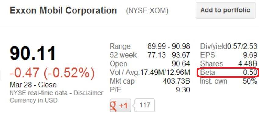
It would also be interesting to compare the values
you obtain for ![]() relative to those reported
by various financial web sites. For example, this is what Google Finance
reports:
relative to those reported
by various financial web sites. For example, this is what Google Finance
reports:
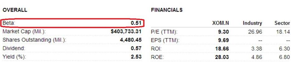
this is
what Reuters reports:
and this
is what Yahoo Finance reports:
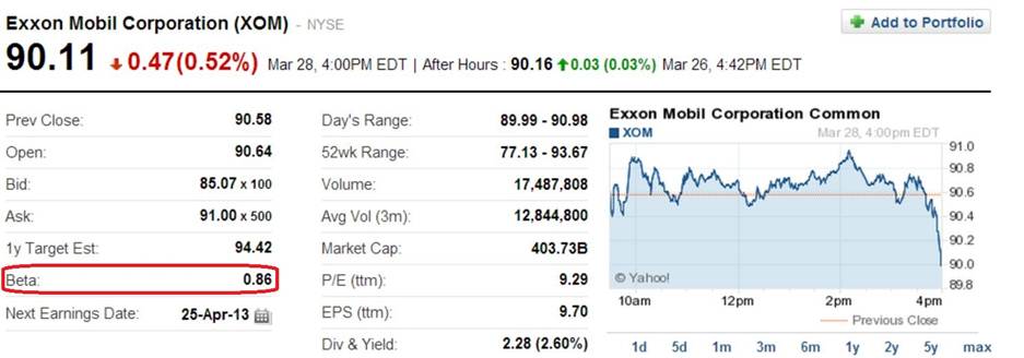
The
‘beta’ values from Google Finance and Reuters are close to the
![]() for Models 1, 2, & 4. The ‘beta’ value from Yahoo Finance is
roughly halfway between the
for Models 1, 2, & 4. The ‘beta’ value from Yahoo Finance is
roughly halfway between the ![]() for Models 1, 2, & 4, and those in Models 3 & 5. What might
account for these differences and similarities? This question is discussed HERE.
for Models 1, 2, & 4, and those in Models 3 & 5. What might
account for these differences and similarities? This question is discussed HERE.
·
You should
also include (and discuss) scatter plots between the excess returns for the
stock you have been assigned and the following variables: (i)
the excess returns on the market portfolio; (ii) the change in risk premium
measure, i.e., the variables ‘crp’; (iii) the size
premium measure, i.e., the variable ‘smb’; and (iv)
the value premium measure, i.e., the variable ‘hml’.
[Note that this means a total of four scatter plots; you can find an
explanation of how to combine these four scatter plots into one graph HERE]. Recall the distinction between
‘unconditional’ and ‘conditional’ correlations from the warm-up HW assignment. HERE is a WORD file with the
scatterplots using the ExxonMobil excess returns data.
·
To help you
refer to the population regression models to be estimated for the paper, HERE is a WORD file with these models
written using the WORD equation editor; you may copy & paste these as you
wish for your paper.
·
Remember:
(a) to properly reference all sources you use; and (b) NOT TO PLAGIARIZE.
Last updated: April 26, 2013. Link to: Econometrics Home Page.