Economics 3343: Homework Assignment #1
Dr. Philip Rothman
Office: Brewster A-424
Phone: 328-6151 Email: rothmanp@ecu.edu
Due date: Thursday, October 27th. The paper for this assignment needs to be submitted at the start of class that day; submission by e-mail will NOT be accepted.
The purpose of this assignment is to run through
a set of exercises with the econometrics software package EViews to help prepare you for your course paper; your grade on this
assignment will be a component of the grade you receive on the course paper.
You can access EViews through one of three ways: (a) at the Kim Lab (Brewster
D-213/214); (b) remotely through ECU’s Virtual Computing Lab (follow the ‘Connect to
VCL’ link and subsequent instructions, and once you’re in the VCL, click on the
‘EViews 8’ link); or (c) with a ‘student version’ bought directly through EViews.
There are two parts to this
assignment. For Part I, you will NOT have to hand in anything for the assignment. However, going
through these steps will be VERY important preparation for your course paper/project. For Part II,
you will have to prepare material to be handed in.
PART I: Becoming Familiar with EViews (There’s Nothing To “Hand In” From Part I)
You can find a set of EViews tutorials AT THIS LINK. EViews is an econometrics
software package. It organizes data, graphs, output, and so forth, as objects.
Each of these objects can be copied, saved, cut-and-pasted into other Windows
programs, or used for further analysis. A collection of objects can be saved
together in a workfile.
I.1 CREATING A GROUP AND SCATTERPLOT
Suppose you want to create a scatterplot
between variables called y and x. To do so, it’s helpful to create an EViews group that contains the two variables.
To do this:
1.
Select the two
variables y and x keeping the “Ctrl” key pressed and left-clicking on the series with
your mouse pointer.
2.
Then right-click with the mouse and select Open > As Group.
3.
To save the group within the workfile, click Name. EViews will offer a default name,
but you can use up to 16 alpha-numeric characters for the name. The click OK. Note: this stores the graph/group in
the workfile, but the workfile also needs to be saved by clicking File > Save > OK.
Then, to create the scatterplot containing an
estimated regression line between y and x, click View > Graph >
Scatter, and then on the right-side of the window click Fit Lines > Regression Line. Once the
graph appears, click Freeze; when the
‘Auto Update Options’ window opens up, keep the ‘Graph Updating’ button clicked
on ‘Off’ and then click ‘OK’ at the
bottom of the window. The click Name >
OK to store the graph in the workfile. If this is the first graph in the
workfile, EViews will list ‘graph01’ as the default name; you can change this
before clicking ‘OK’. Note: You can’t
create an EViews group with c and resid. Another Note:
The reference to the variables y and x
above is only meant as an example, i.e., those variables must be in the
particular workfile for you to actually execute these commands.
I.2 RUNNING A REGRESSION
Suppose you want to run a regression between y and x, including a constant
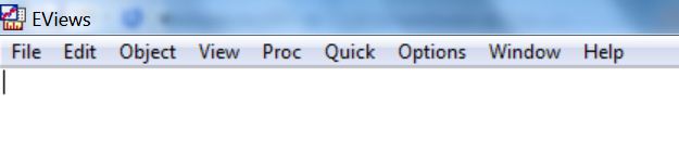
term. You can do so by typing the relevant commands in the EViews command
window, which is the white area just below the EViews menu bar. In this image
the cursor is in the command window, below and a bit to the left of the ‘File’
button:
To run a regression with y as the dependent variable, x as the single independent variable, and a constant term included,
in the command window type ls y c x and then hit ‘Enter’. Here ls
stands for least squares and inclusion of c informs EViews that a constant term should be included in the
model. You can save your regression results in the workfile by clicking Name and then OK. The default name for the first equation to be stored in the
workfile is 'EQ01', and for the second equation it's 'EQ02', etc. Remember that
the workfile also needs to be saved by clicking File > Save.
The regression described above is a simple
regression. Suppose you want to run a regression with a constant with y as the dependent variable and x1 and x2 as the independent variables. To do so, in
the command window type ls
y c x1 x2.
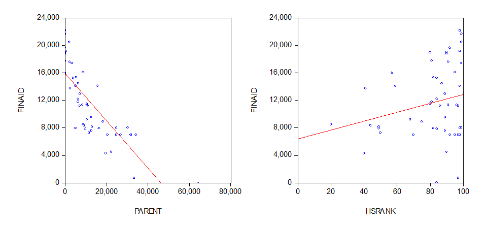
I.3 Equation (2.11)
Equation (2.11) on slide 2-11 of the PPT
slides for Chp. 2 is a regression model estimated with some financial aid data
from a small liberal arts college. Click HERE to
download an EViews workfile with the data used to estimate this regression. The
dependent variable is called finaid, and the two independent variables are parent and hsrank.
Here are scatterplots between the dependent variable and the two independent
variables:
You can create these by:
o
Creating a group between parent and finaid
(click first on parent and then on
finaid), and then following the steps for making a scatterplot with an
estimated regression line included.
o Creating a group between hsrank and finaid
(click first on hsrank and then on
finaid), and then following the steps for making a scatterplot with an
estimated regression line included.
The slopes of the estimated (simple) regression
lines in the scatterplots provide information about the unconditional
correlations between the dependent and independent variables, i.e., the
unconditional correlation between finaid and parent is
negative, and the unconditional correlation between finaid and hsrank is
positive.
To estimate equation (2.11) in EViews after
downloading and opening the workfile, from the command window enter ls finaid c parent hsrank (note that the “l” in “ls” is a lower-case “L”, the letter ‘el’, NOT the number ‘1’) and then hit ‘Enter’. A window
will open up (which when ‘maximized’) looks like the following:
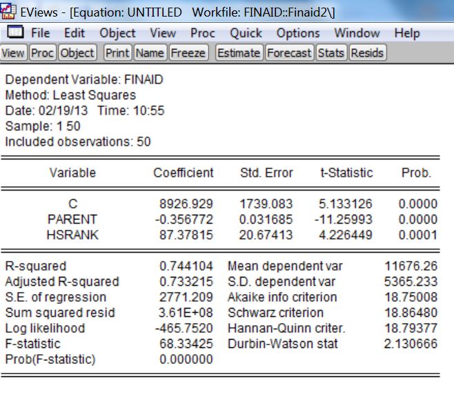
The column
labeled ‘Variable’ has the names of the explanatory variables, PARENT
and HSRANK, with C representing the constant term. The
column labeled ‘Coefficient’ has the values of the estimated coefficients. For
example, the value of the estimated constant term is 8926.929. On the left side of the bottom
section of the window are printed the values of the R-squared and Adjusted
R-squared for the
estimated regression. If you compare the estimated coefficients
with those in equation (2.11), you’ll see that the results are identical. The
signs of the estimated slope coefficients give information about the
conditional correlations between the dependent and independent variables.
PART II: BACK TO THE HOUSING PRICE REGRESSION
At the end of Chp. 1, we discussed an estimated simple regression model for
housing prices in the Los Angeles area. After running through PART I above, you
should be familiar with the basics of (a) getting data into EViews and (b)
running regressions with EViews. The data you'll need for this part of the
assignment are stored in an EViews workfile which can be downloaded by CLICKING HERE.
To open this workfile within EViews click File
> Open > Workfile and then the folder/location you downloaded the
file to. You can find a description of this data set by CLICKING HERE. In the data set are the data used to estimate the housing price
example from Section 1.5. To estimate equation (1.23), you would use the
variable P as the dependent variable and S as the independent variable (and make sure to include a
constant).
Your tasks for Part II are:
1.
While always using the P as the dependent
variable and always including the constant term, estimate regression models by
OLS using the following sets of independent variables:
A.
S N A [from
command line, type ls
p c s n a and then hit
‘Enter’; note that the “l”
in “ls” is a
lower-case letter “L”,
not the number “1”
]
B.
S N A BE [from command line, type ls p c s n a be
and then hit
‘Enter’]
C.
S N A BE BE2 [from command line, type ls p c s n a be be^2 and then hit ‘Enter’]
D.
S N CA SP [from command line, type ls p c s n ca sp
and then hit
‘Enter’]
E.
S CA Y [from command line, type ls p c s ca y
and then hit ‘Enter’]
F.
N A BA Y [from command line, type ls p c n a ba y
and then hit
‘Enter’]
EViews Note: You should save each of these estimated models in your workfile.
The directions for doing so are given in section I.2 of Part I above.
The data are:
·
Pi = the price (in thousands of dollars) of the ith house
·
Si = the size (in square feet) of the ith house
·
Ni = the quality of the neighborhood of the ith house (1 = best, 4 = worst) as rates
by two local real estate agents
·
Ai = the age of the ith
house in years
·
BEi = the number of bedrooms in the ith house
·
BAi = the number of bathrooms in the ith house
·
CAi = a dummy variable equal to 1 if the ith house has central air conditioning, 0 otherwise
·
SPi = a dummy variable equal to 1 if the ith house has a pool, 0 otherwise
·
Yi = the size of the yard around the ith house (in square feet)
2.
Prepare a report/paper to be submitted in
class on Monday, October 20th.
For this report you should:
A.
Include a title page with "Homework
Assignment #1" as the title and including your name and the date.
B.
Present in 'standard format' (as used in the
text) the estimation results for the six alternative housing price models
you've estimated. What is meant by 'standard format'? You can download THIS WORD FILE to see. Note: The
equations in this WORD file were created using the WORD equation editor; within
WORD, the following steps are used to start the WORD equation editor: Insert > Equation.
C.
Present scatter plots (with regression)
between the variable P and each of the
independent variables used in the alternative housing price models; there are
eight such independent variables (excluding BE2): S,
N, A, BE, CA, SP, Y, and BA. For an example of such a plot, you can download THIS WORD FILE. Note: After
creating such a plot/graph in EViews, you can 'copy & paste' the graph into
WORD (by 'inserting' a 'picture' 'From File'. Another Note: Recall that these scatter plots give information
above the ‘unconditional’ correlation between the variables in question. The
sign of a slope coefficient in a model with more than one explanatory variable
gives information about the ‘conditional’ correlation between the dependent
variables and the explanatory variable associated with the slope coefficient
conditional on the other explanatory variables. It is informative to
compare/contrast the unconditional and conditional correlations.
D.
Explain which of the six estimated multiple
models you think is the 'best' model, using the criteria for assessing
estimated regression models we have studied to date (as of 02/18/15) in the
course. Calculus Note: If you’ve had
calculus, you can use the third estimated model to calculate, all else equal,
the number of bedrooms that maximizes the price of the house; it’s interesting
to use that result for the estimated partial effect of ‘BE’ in the second
estimated model.
E.
Structure your paper to have a standard
Introduction-Body-Conclusion format. IN THIS WORD FILE you can find a template to use for a title page and some
suggestions for structuring your paper. Your very important criterion to keep
in mind is the importance of explaining clearly
and exactly to your reader what you have done.
F.
DO YOUR OWN WORK, i.e., DO NOT COPY ANY PART OF ANY
OTHER STUDENT’S PAPER. IF YOU COPY/PLAGIARIZE, YOU WILL COMMIT A VIOLATION OF ECU’s PRINCIPLES OF ACADEMIC INTEGRITY.
Last updated: September
29, 2015.