The use of ecological and social network analysis to study food webs and nutrient cycles in ecological systems that include humans
Joseph J. Luczkovich, Department of Biology, Institute for Coastal and Marine Resources
East
Carolina University, Greenville, NC 27858, luczkovichj@mail.ecu.edu
http://drjoe.biology.ecu.edu
· Many ecological
and social and phenomena can be modeled as networks of interactions.
· For instance, in ecological systems, food webs and nutrient cycles can be represented using species (or groups of similar taxa) as nodes, and flows of energy, carbon, or nitrogen as arcs.In social systems, information, money or other services are the arcs and people (or groups of people) are the nodes in the network.
· At a recent Network Biocomplexity workshop sponsored by the National Science Foundation held in NC (USA), 40 sociologists and ecologists met to discuss the similarity among the approaches used in these two approaches to modeling networks (Science Perspectives article).
· Today, I will discuss the use of network analysis methods to produce models and visualizations of the food webs and nutrient cycle in two systems:
1)· The estuarine seagrass ecosystem at St. Marks, Florida
· Luczkovich, Borgatti, Johnson, Everett (2003),
· Luczkovich, Ward, Johnson, Christian, Baird, Neckles and Rizzo (2002),
· Christian and Luczkovich 1999)
· Map of St. Marks Wildlife Refuge, FL, USA
· Sampling for network analysis at St. Marks
2)
· The Norwegian Nitrogen Cycle (Bleken and Bakken 1997).
· I
will use these examples to display the food web models in a three-dimensional
view of the arcs and nodes, using a multi-dimensional scaling (MDS) of the
nodes to arrange them in space.
· The MDS is based
on the similarity of the nodes in terms of their ecological (trophic) role.
· The trophic role is measured using an algorithm called Regular Equivalence (REGE) in a social network analysis package called UCINET, in which two nodes are judged to be similar if they consume prey of the same REGE class and have predators that are from the REGE class.
· The algorithm is expressed as follows (from Luczkovich et al, in press):
· We represent community food web data as a directed graph, or digraph, G(V,E), which consists of a set of nodes V (also known as vertices) representing species or compartments, and a set of directed ties (also known as edges or arcs) E which represent predation, parasitism or any other trophic relationship.
· The notation (a,b) Î E indicates the presence of a tie from a to b. Similarly, (b,a) Î E, indicates a tie from b to a.
· We can also define a real-valued function F on E which assigns a value (such as a quantity of carbon flow) to each tie, so that f(u,v) = .27 would indicate a flow of .27 units of carbon or nitrogen from u to v.
· The set of nodes adjacent to a given node v is called the neighborhood of v and denoted N(v).
· In a directed graph, a node’s neighborhood consists of two parts:
· an out-neighborhood, defined as the set No(v) = {p| (v,p) Î E}, and
· an in-neighborhood, defined as the setNi(v) = {q | (q,v) Î E}.
· In the case of food web predation data, the out-neighborhood No(u) is the set of species that are predators of species u, and the in-neighborhood Ni(u) is the set of species that are prey of species u.
· An equivalence relation R of a digraph G(V,E) is regular if, for all nodes u,v Î V, uº v implies that if there exists a tie (u,y) Î E, then there exists a node z such that (v,z) Î E and y ºz, and if there is a tie (p,u) Î E, then there exists a node q such that (q,v) Î E and p º q.
· In other words, in a regular equivalence, if nodes u and v are equivalent, then if one has a tie to a third party, then the other one has a corresponding tie to an equivalent third party (but not necessarily the same one).
· Applied to food webs, this means that regularly equivalent species prey on equivalent species and are preyed upon by equivalent species.”
· A
simple example:
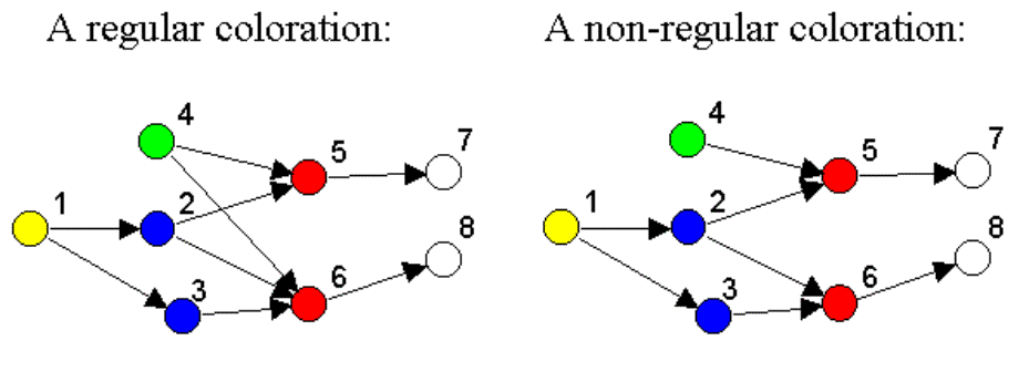
· On
the right diagram, nodes 5 and 6 are NOT regularly equivalent, because they do
not have the same in-neighborhood (blue, green for node 5; blue for node 6)
· The REGE
algorithm assigns species or taxa to classes based on this iterative and
recursive method, starting with all taxa in the same class (for details of the
algorithm, see Luczkovich et al, in press).
· In
the first iteration, the producers (plants, algae) are placed in their own
class (green) because they are consumed by other species but they are not
consumers [Fig. 1; the Appendix below lists the taxa and their numerical
codes].
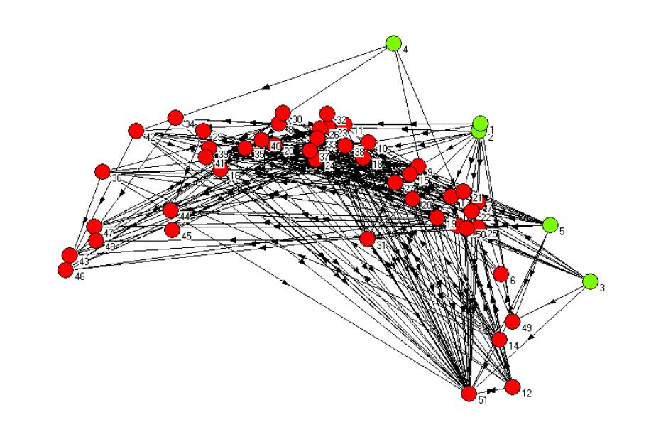
Figure 1. The non-metric multi-dimensional scaling plot of the
St. Marks carbon flow food web network after 1 iteration of the REGE algorithm,
with plants and algae shown as a separate group (green nodes).
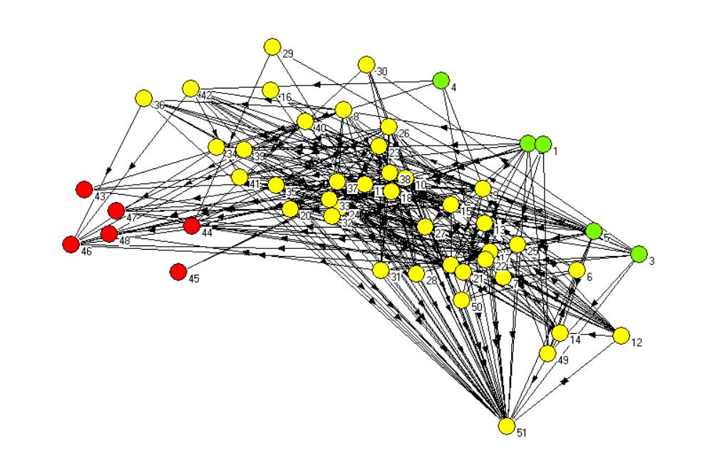
Figure 2.The non-metric multi-dimensional scaling plot of the
St. Marks carbon flow food web network after 2 iterations of the REGE
algorithm, with plants and algae shown as green nodes, top-carnivore (birds)
shown in red.Yellow nodes are all the remaining taxa, which are intermediate
consumers.Node 51 is detritus (sediment particulate organic carbon).
· After
51 iterations, there are ten classes with REGE coefficients that exceed a
cut-off level of REGE coefficients [Fig. 3].

· Thus, any two nodes are similar if they plot together in space, and very different if the plot far apart in space.
· At the workshop, using MAGE, a software package for visualization of molecular models, I will display the three-dimensional model of the St. Marks seagrass ecosystem carbon flow food web.
· Finally, I will display a similarly derived network model of the N-Cycle of Norway.
· Bleken and Bakken (1997) examined the nitrogen involved in the food production system of Norway.In this work, the authors analyzed the nitrogen flows within Norway’s society and their dissipation into the environment.
· In their analysis, the food-producing sectors of society had the greatest interaction with other aspects of the nitrogen cycle and the largest nitrogen flow.
· For example, in their Figure 1, the “wholesale food supply” compartment had flows into it that summed to 26.1 Gg of N per year.Other compartments with large flows included plant production (126 Gg of N per year) and animal production (101.5 Gg of N per year).
· I performed a network analysis of these data using the regular equivalence (REGE) approach outlined described above on these data, which groups compartments together in 3 dimensions based on their similar roles (and similar flows) in the nitrogen cycle.
· The
resulting nitrogen network diagram [Fig. 4] is arranged so that low
trophic-level compartments (such as“synthetic fertilizer”, ”fishing industry”
and “sea catch” where N comes into the system) are at the bottom and high
trophic-level compartments are at the top and outside of the diagram.
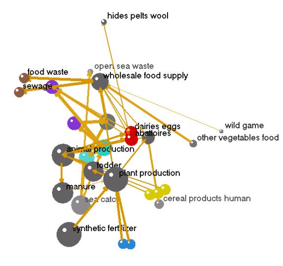
· Nodes associated with waste (“sewage”, “food waste”, and “open sea waste”) are all located near the top and outside of this 3D graph of the network, suggesting that these compartments are the way N is exported from the system.
· One interesting conclusion of visualizing the Bleken and Bakken (1997) data in this way is that one can appreciate the very large role “synthetic fertilizer” plays in the production of food in Norway, much larger than the nitrogen arising from “biological fixation” and “atmospheric deposition”.Although this source of nitrogen has always been assumed to play a significant role, unlike a traditional box and arrow diagram, the relative size of the nodes in this network visually communicate the relative importance of the nodes.
· Node radii (ball sizes) are scaled according to the log-transformed amount of nitrogen contained in each node.
· The thicknesses of the arrows also represent the magnitude of the flows among nodes (log-transformed flows).
· The nodes for “plant production”, “fodder”, “animal production” and the “wholesale food supply” are large and show a distinct dominant pathway leading from synthetic fertilizers to human consumption.
· Other nodes are instantly visualized as less significant, such as “wild game” and “open sea waste”.
· This method does not depend on an artist’s placement of the nodes or the approximation of the size of a node, as is almost always the case in a traditional flow model using boxes and arrows.
· The UCINET and MAGE software are all that are required for a visualization of the network that is closely related to the quantitative mass flows of nitrogen in Norway.
· The convenience and power of the new visualization software enables public citizens, educators, students, farmers, politicians and environmental managers to view and easily interpret complex biogeochemical data.
· The complex nature of this food web and the nitrogen sources and fates of food production in Norway is more easily appreciated using such visualizations.
Conclusions
· In both of these
models, the size of the nodes has been made proportional to the amount of
carbon or nitrogen passing through the node.
· So, for example, in the Norwegian N-Cycle, one can see that much of the nitrogen passing through the food web is coming from synthetic fertilizer and ends up as sewage and food waste.
· In the St. Marks model, the main source of carbon for the food web is detritus.
· Comparisons among different food webs made at different times are thus possible.
· The pathways by which nutrients flow and are stored in these food webs can be visualized using REGE and MDS display of the network.
· This visualization approach can be used to explore relationships among nodes and aid in the understanding of complex phenomena in social and natural systems.
· In the future, the use of the network analysis approach will allow us to model and visualize the effects humans can have on the food webs of global ecosystems.
Appendix1:A list of the identification
codes and compartment names for the St. Marks seagrass carbon flow food web
taken from Baird et al. (1998).See Christian and Luczkovich (1999) for a
complete species list within each compartment.
(1) Phytoplankton,
\-
algae, (6) Bacterio-plankton,
(7) Micro
protozoa, (8) Zooplankton,
(9) Epiphyte-grazing amphipods,
(10) suspension-feed
molluscs, (11) Suspension-feed
polychaetes , (12) Benthic
bacteria, (13) Micro fauna, (14) Meiofauna,
(15) Deposit-feeding
amphipods, (16) Detritus-feeding crustaceans, (17) Hermit crab, (18) Spider
crab, (19) Omnivorous crabs,
(20) Blue crab,
(21) Isopod, (22) Brittle
stars, (23) Herbivorous
shrimp, (24) Predatory shrimp,
(25) Deposit-feeding
gastropod, (26) Deposit-feeding
polychaetes, (27) Predatory
polychaetes, (28) Predatory
gastropod, (29) Epiphyte-grazing gastropod, (30) Other gastropods, (31) Catfish and stingrays, (32) Tonguefish , (33) Gulf
flounder & needle fish, (34) Southern hake & sea robins, (35) Atlantic silverside &
bay anchovies, (36) Gobies
& blennies, (37) Pinfish,
(38) Spot, (39) Pipefish & seahorses,
(40) Sheepshead
minnow, (41) Red
Drum, (42) Killifish,
(43) Herbivorous ducks,
(44) Benthos-eating
birds, (45) Fish-eating
birds, (46) Fish & crustacean eating birds, (47) Gulls, (48) Raptors,
(49) Dissolved Organic Carbon (DOC), (50) Suspended Particulate Organic Carbon,
(51) Sediment POC
References
Baird, D., Luczkovich, J. J. and Christian, R. R.(1998) Assessment of spatial and temporal variability in ecosystem attributes of the St. Marks National Wildlife Refuge, Apalachee Bay, Florida. Estuar. Coast.Shelf Sci. 47, 329-349.
http://drjoe.biology.ecu.edu/publications/ECSS_Vol47.PDF
http://drjoe.biology.ecu.edu/publications/EcologicalModeling_117pp99-124.PDF
http://drjoe.biology.ecu.edu/publications/Science_mag_08_31_01.pdf